Estimating shading across the BCI 50-ha plot
I calculated summed vegetation density above points in the forest using the method described in several papers by Ruger et al (all available here). In canopy surveys prior to 1997, presence-absence of vegetation in contact with a vertical line was recorded; the calculation presented here up to 1983 are based on those data, and exactly match the data in Ruger et al. Since 2003, however, the method changed, vegetation density was estimated in voxels of 5x5 m horizontally by the standard vertical profile, with a sliding score given between 0 and 100. I initially made of the scores between 0 and 100 in each voxel to repeat the Ruger method, however, these worked poorly. There were substantial differences between observers, and even among different locations done by the same observer in the same year. So I reverted to the earlier calculation method, using only presence-absence: a voxel either had no vegetation at all (score 0), or some vegetation (score > 0). Note, though, that the method prior to 1997 and since 2003 are still not exactly comparable, because in early censuses, vegetation was only scored along a vertical line, whereas in later censuses it was considered in an entire three-dimensional cell.
Prior to 1997, there were no missing values, but in 2003, 2008, 2010, a few coordinates had no canopy data. To fill in the map, I randomly assigned the missing values to either presence or absence using a random draw from a binomial distribution with probability equal to the proportion of points with vegetation in the same layer and the same year.
In the Ruger et al. papers, the summed vegetation density above a point was referred to as a shade index: the more vegetation, the denser the shade. I ran the calculation of this shade index at the middle of every 5x5 m grid in the 50-ha plot (excluding 27.5-m edges), using a height of 0.5 m above the ground, repeating this in all years 1983-1994, 1996, and 2003-2012. The 1985-1989 shade estimates were used in Ruger et al., though from a height of 2 m, not 0.5 m.
Results can be downloaded in R format here. All are in a single table, with one row per point.
| x | y | recruit10 | recruit90 | s1985 | s1986 | s1987 | s1988 | s1989 | s1990 | s2005 | s2006 | s2007 | s2008 | s2009 | shade8589 | shade0509 | |
|---|---|---|---|---|---|---|---|---|---|---|---|---|---|---|---|---|---|
| 1 | 27.50 | 27.50 | 0.00 | 0.00 | 119.90 | 113.77 | 128.22 | 115.58 | 118.34 | 126.90 | 152.96 | 175.37 | 187.97 | 189.03 | 183.94 | 119.16 | 177.85 |
| 2 | 27.50 | 32.50 | 0.00 | 2.00 | 118.08 | 111.23 | 127.59 | 115.16 | 116.54 | 126.75 | 152.64 | 175.39 | 187.60 | 188.88 | 183.71 | 117.72 | 177.64 |
| 3 | 27.50 | 37.50 | 0.00 | 2.00 | 115.13 | 109.26 | 125.51 | 113.60 | 114.48 | 125.23 | 150.31 | 173.05 | 184.83 | 186.42 | 181.19 | 115.60 | 175.16 |
| 4 | 27.50 | 42.50 | 0.00 | 0.00 | 114.08 | 103.38 | 124.50 | 115.28 | 116.25 | 131.05 | 143.73 | 167.11 | 177.95 | 178.97 | 172.70 | 114.70 | 168.09 |
| 5 | 27.50 | 47.50 | 1.00 | 1.00 | 114.34 | 103.58 | 125.01 | 116.68 | 118.06 | 132.34 | 145.40 | 168.99 | 179.90 | 181.18 | 174.86 | 115.54 | 170.07 |
| 6 | 27.50 | 52.50 | 1.00 | 3.00 | 112.94 | 103.26 | 123.85 | 115.90 | 117.84 | 131.84 | 145.21 | 168.62 | 179.65 | 180.99 | 174.70 | 114.76 | 169.84 |
Recruitment per 5x5 correlates negatively with the mean shade index over 1985-1989. This was the basis of Ruger et al. The correlation coefficient is \( -.219 \). For 2005-2009, the correlation is also negative, though the coefficient is much weaker at \( -.103 \). Apparently the shade index in 2005-2009 is registering something relating to light.
| recruit90 | recruit10 | shade8589 | shade0509 | |
|---|---|---|---|---|
| recruit90 | 1.000 | 0.003 | -0.219 | -0.060 |
| recruit10 | 0.003 | 1.000 | -0.033 | -0.105 |
| shade8589 | -0.219 | -0.033 | 1.000 | 0.598 |
| shade0509 | -0.060 | -0.105 | 0.598 | 1.000 |
The correlation between recruitment and shading shows up with an estimate of the mean density of recruits (per 5x5) in the four quartiles of shade. In 1990, there was nearly double the recruitment in the areas in the lowest quartile of shade:
| lowest quartile | medlow quartile | medhigh quartile | highest quartile | |
|---|---|---|---|---|
| shade | [75.6,108) | [108,115) | [115,123) | [123,148) |
| recruits | 2.614 | 1.902 | 1.671 | 1.315 |
In 2010, recruitment was likewise higher in the lowest quartile of shade, but by only about 60%:
| lowest quartile | medlow quartile | medhigh quartile | highest quartile | |
|---|---|---|---|---|
| shade | [135,167) | [167,177) | [177,186) | [186,214) |
| recruits | 1.637 | 1.467 | 1.243 | 1.034 |
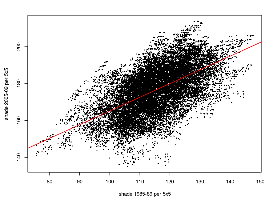
The correlation between 1980s shade and 2000s shade is remarkably strong.
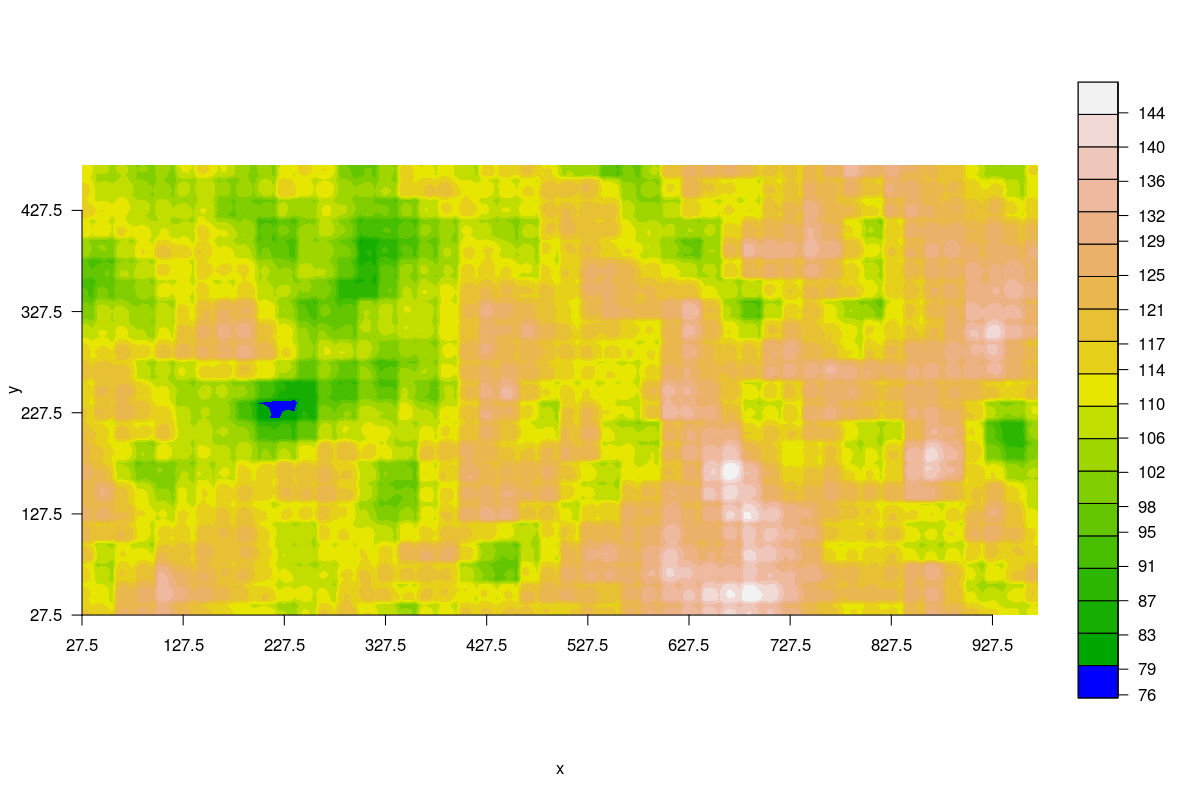
Maps of shade show how the pattern of shade across the plot remained consistent.
Shade index averaged over 1985-1989.
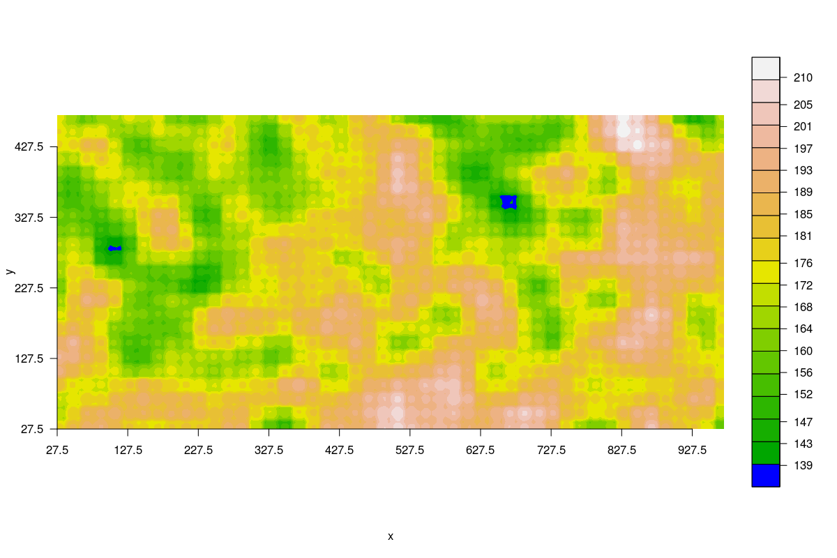
Shade index averaged over 2005-2009.
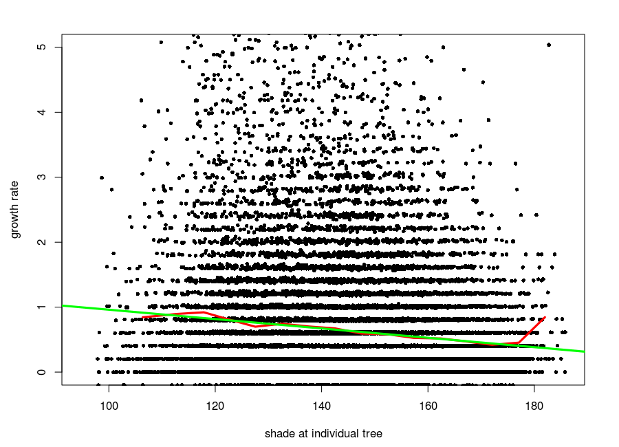
Next I calculated the shade index at the tops of trees alive in the 2005 census in the years 2005-2009. The heights of trees were calculated using height allometry parameters estimated long ago and appearing in Supplementary Material in the Chave biomass paper (as they were in Ruger's papers). The shade estimates can be downloaded in R format here. It is a single table, with one row per tree, giving the species name, coordinates, dbh, a shade estimate each year, then the mean shade over 5 years.
I then calculated diameter growth rate over 2005-2010 for those trees using the growth.indiv function in the CTFS R Package. Growth is negatively correlated with the shade index.