Finding land use categories inside polygons of a town
The goal is combining the land-use GIS and the metropolitan areas around Chicago in order to compare land use in various towns. This will require manipulating two kinds of GIS in ways we reviewed 18-25 Oct. The large land-use raster should be cropped down, then it must be combined Chicago GIS, requiring identical coordinate systems (the projection).
The raster GIS lcoi_99-00b.tif gives land-use categories across all Illinois. Categories are defined at here. In a raster class, the slot crs shows the projection. You must remember that slots are accessed with the @:
library(raster)
LandUse=raster('lcoi_99-00b.tif')
Cropping is most easily down using the raster function drawExtent, then clicking on the map to surround Chicago. Saving the output produces an Extent object with four corners.
plot(LandUse)        ## Graph omitted
ChiBox=drawExtent()
ChiBox
class       : Extent
xmin        : 380547.6
xmax        : 461105.5
ymin        : 4588527
ymax        : 4706936
ChiLandUse=crop(LandUse,ChiBox)
plot(ChiLandUse) ## Graph omitted
The raster package includes convenient tools for getting at the data. The following steps can be used to convert any raster into a dataframe with columns for coordinates and the land use score.
landcat=getValues(ChiLandUse)
ChiLandUseCoord=xyFromCell(ChiLandUse,cell=1:length(landcat))
ChiLandUseDF=data.frame(ChiLandUseCoord,landcat)
head(ChiLandUseDF)
         x       y landcat
1 380557.2 4706932      14
2 380587.2 4706932      14
3 380617.2 4706932      14
4 380647.2 4706932      11
5 380677.2 4706932      12
6 380707.2 4706932      11
Now the municipalities GIS must be aligned into the same projection. I downloaded Chicago GISes from the Chicago Data Portal, and have prj files. What I just learned is that readShapePoly does not capture the prj, while readOGR from the rgdal library does, saving it in the proj4string slot. It has the same information as raster's slot crs. So it is a big advantage getting rgdal working and using readOGR. To learn more about projections, you could look at the Spatial Reference web page or notes from NCEAS (where I first studied this).
library(maptools)
library(rgdal)
Cities=readShapePoly('Municipalities')
CitiesOGR=readOGR('','Municipalities')   ## Notice that readOGR takes first a folder then a file as the arguments to read a set of GIS files
Once the projections are known and stored for two different GISes, the transformation works easily. To switch a Spatial Class, such as Shape Polygons (created by readShapePoly and by readOGR, the function is spTransform. Here, CitiesOGR has its projection properly named (slot proj4string), and ChiLandUse has one too (slot crs):
ChiLandUse@crs
CRS arguments:
 +proj=utm +zone=16 +datum=NAD83 +units=m +no_defs +ellps=GRS80 +towgs84=0,0,0
Cities@proj4string
CRS arguments: NA
CitiesOGR@proj4string
CRS arguments:
 +proj=tmerc +lat_0=36.66666666666666 +lon_0=-88.33333333333333 +k=0.9999749999999999 +x_0=300000 +y_0=0 +datum=NAD83 +units=us-ft +no_defs +ellps=GRS80 +towgs84=0,0,0
CitiesUTM=spTransform(CitiesOGR,ChiLandUse@crs)
Now you can test by plotting to show the two GISes overlay correctly.
plot(ChiLandUse)
plot(CitiesUTM,add=TRUE)   ## Graph omitted
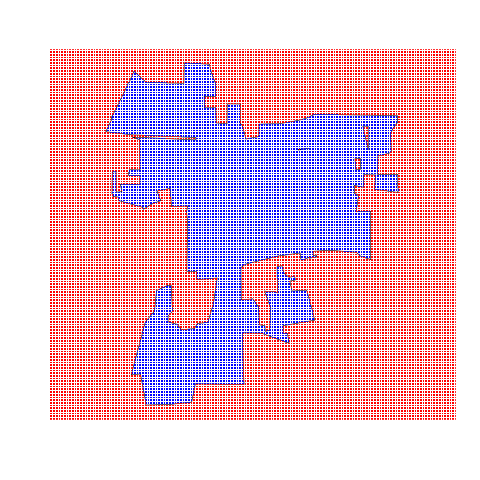
To count land use categories in one municipality, it is quickest (and most accurate) to take advantage of features built-in to the Spatial Classes. Emma discovered this last week... This requires converting the raster object to a Spatial Points Class, which starts with the data frame and coordinates created from the raster. It takes just one step, using the maptools function SpatialPointsDataFrame, passing it the table of coordinates, the table of data (having the land use column), and the projection. Once it is converted to this Spatial Class (check its class), it is then just one step to extract all the points within any Spatial Polygons class. You can confirm this by plotting maps. The step of extracting land use points wihin a town is rather slow. I will leave until later procedures that might speed this up.
landusePt=SpatialPointsDataFrame(coords=ChiLandUseCoord,data=ChiLandUseDF,proj4string=ChiLandUse@crs)
class(landusePt)
[1] "SpatialPointsDataFrame"
attr(,"package")
[1] "sp"
lislepoly=subset(CitiesUTM,NAME=='Lisle')
landuseLisle=landusePt[lislepoly,]           ## This is a very convenient tool: find all points in the landuse Points class that are inside all polygons of one city
landcatsLisle=landuseLisle@data$landcat
table(landcatsLisle)
landcatsLisle
  11   12   14   21   25   31   32   35   41   42   44   51
  42    4    2 1771  457 2200 8932 4922  150   38   17  255
sp::plot(lisle)
points(y~x,data=landusePt@coords,pch='.',col='red')
points(y~x,data=landuseLisle@coords,pch='.',col='blue')
