R GIS for raster data
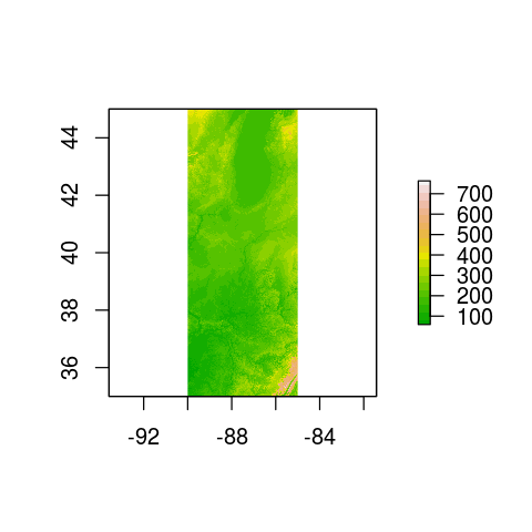
The package named raster has many tools for reading, manipulating, and mapping raster data. Just like the Spatial Classes for polygons, it works with Spatial Classes for raster, and these allow easy loading mapping without any understanding of what's inside. Below, the function raster creates a RasterLayer class using special geotiff files for world topography. These srtm elevation files (90-m topography for the entire world) are available here in chunks of 5x5 degrees . Panama happens to span two pieces, which is why I use two below, with the function merge to combine them. The data below are huge -- two files with 36 million points each -- and your computer may encounter slow downs trying to use it. In the commands below, I remove the first two objects after merging to reduce the strain on R's memory. Cropping the data to a smaller size is easy with raster, and the steps below move right there.
library(raster)
rast04=raster('srtm_19_04.tif')
rast05=raster('srtm_19_05.tif')
allIll=merge(rast04,rast05)
class(rast04)
[1] "RasterLayer"
attr(,"package")
[1] "raster"
slotNames(rast04)
[1] "file" "data" "legend" "title" "extent" "rotated" "rotation" "ncols" "nrows" "crs" "history" "z"
str(rast04@extent)
Formal class 'Extent' [package "raster"] with 4 slots
  ..@ xmin: num -90
  ..@ xmax: num -85
  ..@ ymin: num 40
  ..@ ymax: num 45
rast04@extent
class       : Extent
xmin        : -90.00042
xmax        : -84.99958
ymin        : 39.99958
ymax        : 45.00042
rast04@nrows
[1] 6001
rast04@ncols
[1] 6001
rm(rast04)
rm(rast05)
allIll@extent
class       : Extent
xmin        : -90.00042
xmax        : -84.99958
ymin        : 34.99958
ymax        : 45.00042
class(allIll)
[1] "RasterLayer"
attr(,"package")
[1] "raster"
plot(allIll,col=terrain.colors(20))

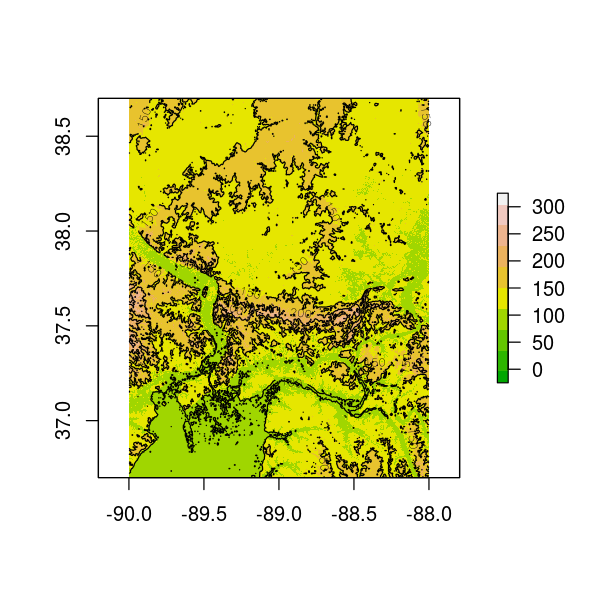
To zoom, you first plot, then run zoom. To crop, you need to create an Extent object, what raster calls a bounding box. There is a function called drawExtent() to create an extent by clicking on the map. Note that you must click on the map after executing! Nothing happens until you click.
zoom(allIll)
ext=drawExtent()
ext
You can also create an Extent object manually.
SIllExt=extent(-90,-88, 36.7, 38.7)
SIll=crop(total,SIllExt)
plot(SIll,col=terrain.colors(10))
contour(SIll,add=TRUE,levels=c(50,100,150,200,250,300,350))

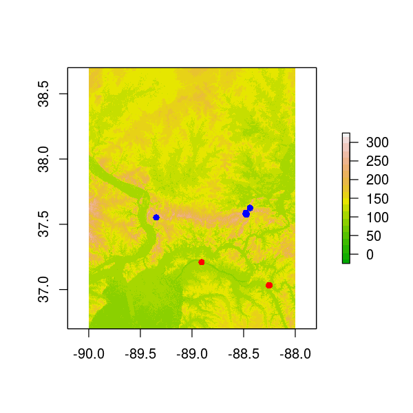
The package includes straightforward tools for getting at the data. This makes it possible to explore the data, for example to find the points where elev<0 (must be errors in the satellite data), or the highest points.
elev=getValues(SIll)
length(elev)
[1] 5760000
summary(elev)
   Min. 1st Qu.  Median    Mean 3rd Qu.    Max.
  -93.0   115.0   134.0   135.4   152.0   327.0
coord=xyFromCell(SIll,cell=1:length(elev))
xyz=data.frame(coord,elev)
head(xyz)
          x        y elev
1 -89.99917 38.69917  154
2 -89.99833 38.69917  148
3 -89.99750 38.69917  145
4 -89.99667 38.69917  148
5 -89.99583 38.69917  151
6 -89.99500 38.69917  151
summary(xyz)
       x               y             elev
 Min.   :-90.0   Min.   :36.7   Min.   :-93.0
 1st Qu.:-89.5   1st Qu.:37.2   1st Qu.:115.0
 Median :-89.0   Median :37.7   Median :134.0
 Mean   :-89.0   Mean   :37.7   Mean   :135.4
 3rd Qu.:-88.5   3rd Qu.:38.2   3rd Qu.:152.0
 Max.   :-88.0   Max.   :38.7   Max.   :327.0
plot(SIll,col=terrain.colors(20))
points(y~x,subset(xyz,elev<(-0)),col='red',pch=16)
points(y~x,data=subset(xyz,elev>300),col='blue',pch=16)

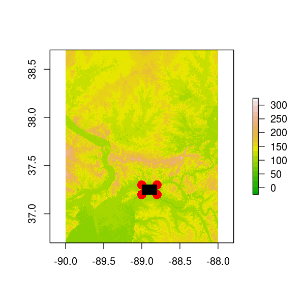
A useful function for raster data is point.in.polygon in the sp package. This example starts with a square polygon, creating a dataframe with four corners. Passing all the points from the raster and the one polygon produces a vector of one value per point, in this case __, equal to 1 if the point is inside, 0 if it's outside. A more useful example would be to use a polygon such as a national park; then you could explore elevation only within the park. The splancs package also has a function to test which points are inside a polygon: inout, inpip, pip.
samplepoly=data.frame(x=c(-89,-89,-88.8,-88.8),y=c(37.2,37.3,37.3,37.2))
samplepoly
      x    y
1 -89.0 37.2
2 -89.0 37.3
3 -88.8 37.3
4 -88.8 37.2
test=point.in.polygon(point.x=xyz$x,point.y=xyz$y,pol.x=samplepoly$x,pol.y=samplepoly$y)
table(test)
test
      0       1
5731200   28800
plot(SIll,col=terrain.colors(20))
points(y~x,samplepoly,col='red',pch=16,cex=2)
points(y~x,data=subset(xyz,test==1),pch=16,cex=.1)

Try mapping land-use categories in Illinois from U of I Prarie Research Institute. Check the crs slot of rasters.
land=raster('lcoi_99-00b')
Here is how to convert to lat-long. Copying the lines should work (though very slowly), but truly understanding is a more advanced topic. This borrows the crs slot of the raster allIll. The function projectRaster comes with the package. It does all the work.
land=raster('~/meetings_workshops/Rgis/data/lcoi_99-00b.tif')
landLatLong=projectRaster(land,crs=allIll@crs@projargs)